import pandas as pd
import matplotlib.pyplot as pltTempreture Derivatives
HDD vs CDD
The term HDD stands for Heating Degree Days, and CDD stands for Cooling Degree Days. Both are used to estimate the energy required to heat or cool an environment.
\[ HDD = \sum_{i=1}^{n} \max(0, T_{base} - T_{avg}) \]
\[ CDD = \sum_{i=1}^{n} \max(0, T_{avg} - T_{base}) \]
Where:
- \(T_{base}\) is the base temperature, which is the temperature below which the building needs to be heated or above which the building needs to be cooled.
- \(T_{avg}\) is the average temperature for the day. In EU, the base tempreture is usually 15.5°C and in US it is 65°F (18.3°C).
Use the Sample Data
weather_data = pd.read_excel("data_weather.xls")weather_data.info()<class 'pandas.core.frame.DataFrame'>
RangeIndex: 2923 entries, 0 to 2922
Data columns (total 4 columns):
# Column Non-Null Count Dtype
--- ------ -------------- -----
0 Time 2923 non-null datetime64[ns]
1 min 2923 non-null float64
2 max 2923 non-null float64
3 mean 2923 non-null float64
dtypes: datetime64[ns](1), float64(3)
memory usage: 91.5 KBweather_data.describe()| Time | min | max | mean | |
|---|---|---|---|---|
| count | 2923 | 2923.000000 | 2923.000000 | 2923.000000 |
| mean | 2014-07-30 00:00:00 | 52.889648 | 66.726300 | 58.481250 |
| min | 2010-07-30 00:00:00 | 35.400000 | 43.500000 | 41.643182 |
| 25% | 2012-07-29 12:00:00 | 49.000000 | 61.900000 | 54.324404 |
| 50% | 2014-07-30 00:00:00 | 53.100000 | 65.500000 | 58.078986 |
| 75% | 2016-07-29 12:00:00 | 56.300000 | 71.100000 | 62.006349 |
| max | 2018-07-30 00:00:00 | 73.400000 | 107.500000 | 86.555390 |
| std | NaN | 5.412125 | 7.879157 | 5.561259 |
weather_data = weather_data.set_index("Time")
weather_data.plot(figsize=(12, 6))
plt.show()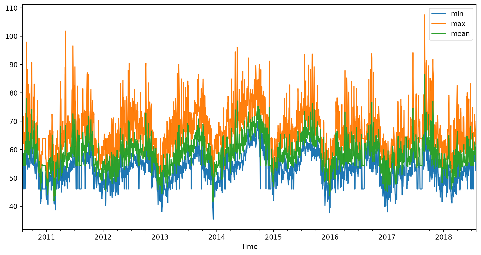
plt.figure(figsize=(12, 6))

plt.hist(weather_data['min'], bins=60, alpha=0.5, label='Min')
plt.hist(weather_data['max'], bins=60, alpha=0.5, label='Max')
plt.hist(weather_data['mean'], bins=60, alpha=0.5, label='Mean')

plt.title('Histogram of Min, Max, and Mean Values')
plt.xlabel('Values')
plt.ylabel('Frequency')
plt.legend()

plt.show()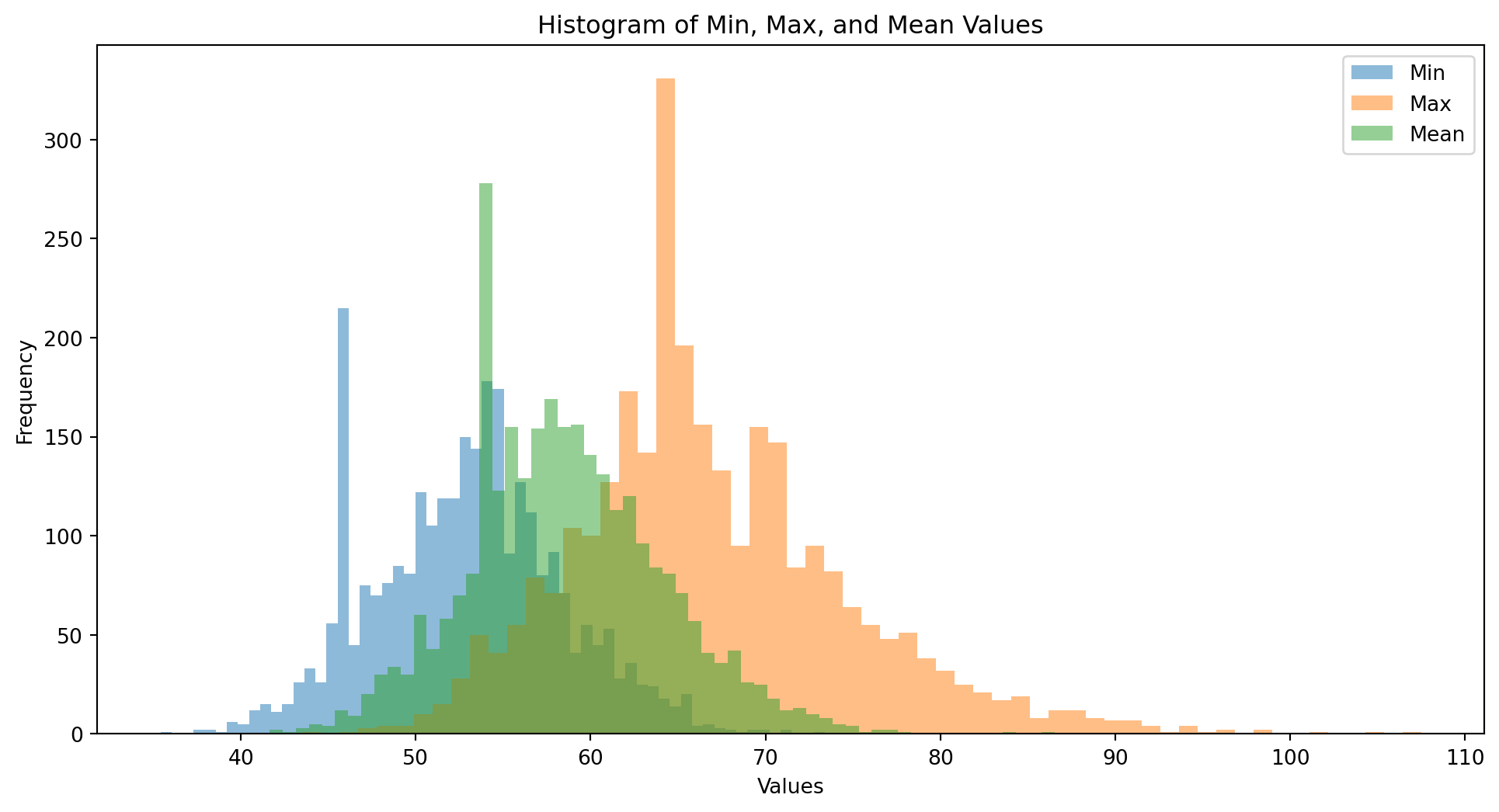
winter_filter = (weather_data.index.month == 12) | (weather_data.index.month == 1) | (weather_data.index.month == 2)
winter_data = weather_data[winter_filter]

summer_filter = (weather_data.index.month == 6) | (weather_data.index.month == 7) | (weather_data.index.month == 8)
summer_data = weather_data[summer_filter]
# histogram of winter and summer data
plt.figure(figsize=(12, 6))
plt.hist(winter_data['mean'], bins=60, alpha=0.5, label='Winter Mean')
plt.hist(summer_data['mean'], bins=60, alpha=0.5, label='Summer Mean')
plt.title('Histogram of Winter and Summer Mean Values')
plt.show()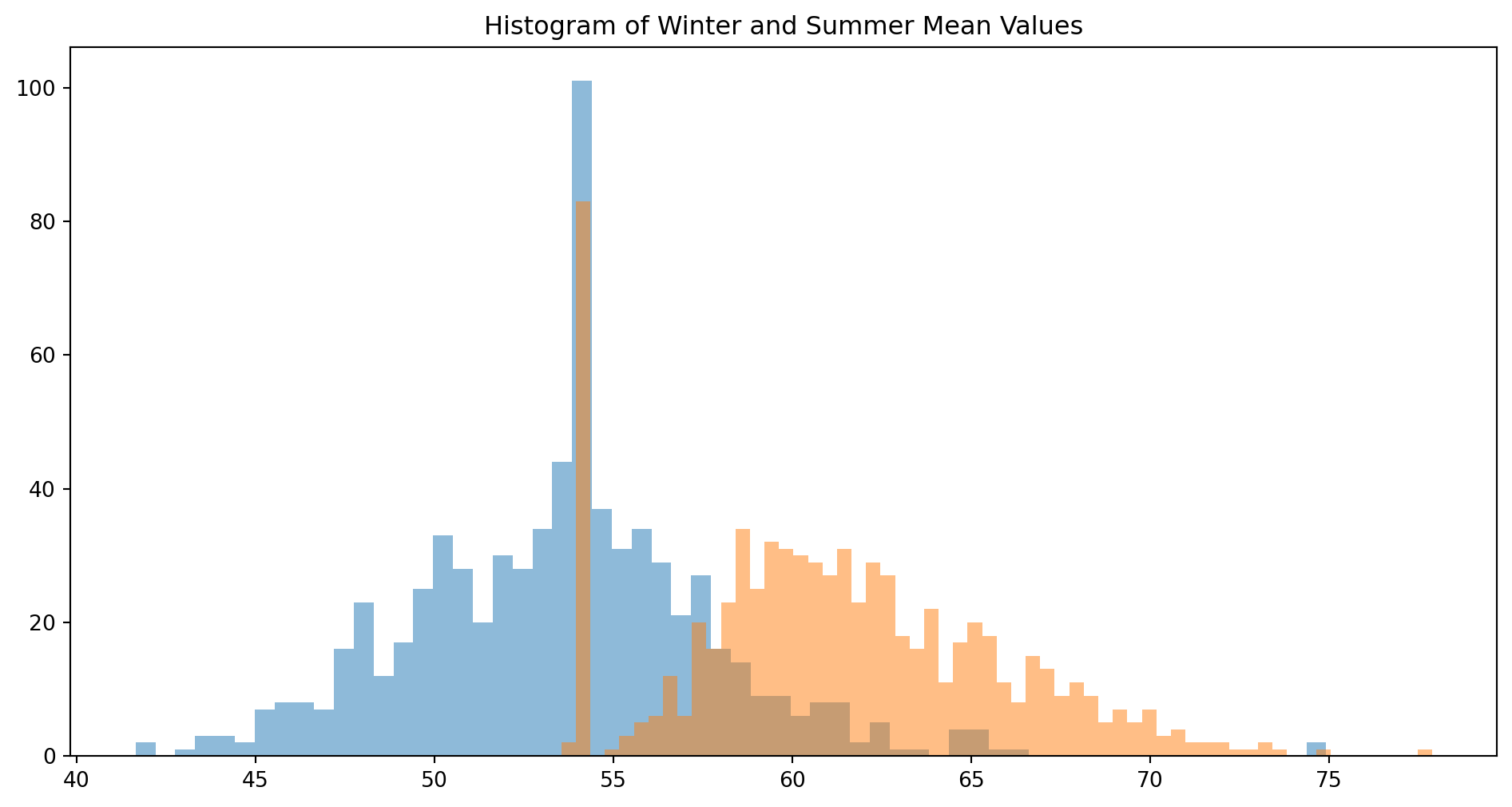
Modeling Tempereature
Our model will be specified as \[ d T_t=\left\{\frac{d T_t^m}{d t}+\alpha \left(T_t^m-T_t\right)\right\} d t+\sigma_t d W_t, \quad t>s \] where \(T_t\) is tempereture at \(t\), \[ T_t^m=\underbrace{A+B t}_{\text{liear component}}+\underbrace{C \sin (\omega t+\phi)}_{\text{cyclic component}}, \] \(A\), \(B\), \(C\) and \(\phi\) are parameters. \(T_t^m\) represents mean value, \(\alpha\) is mean-reverting coefficient, \(\sigma\) is volatility of tempereture, \(W_t\) is a Wiener process.
The solution of this PDE is called Ornstein-Uhlenbeck process.
Please refer to the analytical solution of the Ornstein-Uhlenbeck process for more details: https://planetmath.org/analyticsolutiontoornsteinuhlenbecksde
We will use the result directly in our model.
\[ T_t=\left(x-T_s^m\right) e^{-a(t-s)}+T_t^m+\int_s^t e^{-a(t-\tau)} \sigma_\tau d W_\tau, \]
The basic idea is to replace drift term and integrate on the volatility term.